
About this paper
This paper examines how weather, route choice, forecasts, boat performance and rating relate to the Transpac and Pacific Cup. Its elapsed-time, corrected-time, forecast-cycle and between-boat quantities remain separate rather than being added into one causal total.
Abstract
We ask which measurable differences in weather, routing, forecasts and rating are large enough to matter in the Transpac and Pacific Cup. The analysis combines historical routes through ERA5 weather, thirteen tracked race editions, modern ECMWF ensemble forecasts and a public rating-certificate archive. With the boat, course and solver held fixed, we detected no navigationally relevant long-run trend: the fitted change in optimal elapsed time over the satellite era has a 95 % confidence interval of [−9 h, +29 h]. The weather within a race window matters much more. Departures five days apart differ by a mean 26.4 h for the same boat. Division winners did not occupy a different strategic latitude from their rivals: −0.5 nm, 95 % CI [−11.1, +10.2]. When their tracks were replayed against those rivals on the same hypothetical boat, the elapsed-time difference was +0.02 h [−1.12, +1.16]. The winner's recorded track was nevertheless shorter in 49 of 74 comparisons, with a mean difference of −12.0 nm [−22.6, −1.5] (sign-test p = 0.007). Across eligible forecast cycles (60 of 63), selecting a route against all fifty ensemble members rather than the deterministic forecast improved routed time by +1.10 h per cycle [+0.41, +1.92]. Sensitivity scenarios for unscored firings ranged from +0.62 h to +2.06 h, and the pessimistic interval included zero. For nominally identical sister ships, the median within-group rating spread across public certificates is 1.60 %. Because that spread includes genuine configuration differences, it measures configuration-plus-certificate scatter rather than rating error. The archive therefore shows large departure-date variability, no detected change in the long-run route climate, no separate strategic lane occupied by winners and a possible but modest ensemble-management gain. It does not isolate a single causal mechanism for winning.
1. The question
1.1 The route around the High
Draw the shortest line from California to Hawaii. It passes closer to the centre of the North Pacific High than most fast routes do, and the centre is where the wind is light. Sailing north shortens the course but moves the boat toward the ridge. Sailing south adds distance but usually keeps more pressure in the sails. The central navigation problem is deciding how much distance to trade for wind. A second question follows: where do the candidate routes stop reconverging?
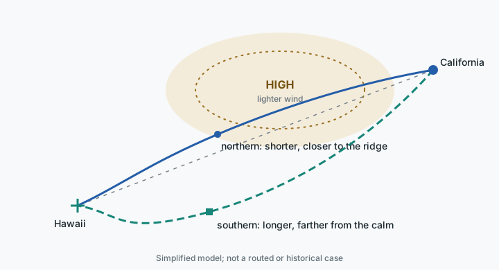
The Transpac runs from Point Fermin to Diamond Head. The Pacific Cup starts about four degrees farther north, in San Francisco, and finishes in Kaneohe Bay. Both are July races. Their boats leave the coastal wind on the High's eastern flank, reach westward into the gradient and gybe into the trades before Hawaii. They are commonly described as downwind races, but they do not begin in the trades.
Stan Honey's published Pacific Cup guidance states the choice plainly: “the most critical decision of the Pacific Cup is where to cross the ridge” (Honey, n.d.-a). It also warns that the costly error is usually to the north. The official Transpac programmes contain three dedicated navigator's guides, in 1995, 2007 and 2021; each prints substantially the same essay. This paper tests that long-standing guidance against reanalysis, forecast replays and tracked fleets.
Both races send groups of divisions off on different days so that boats of different speeds arrive closer together. This paper calls each group a start. A division is the rated class in which a boat competes, and its result is decided on corrected time: elapsed time adjusted by the boat's rating. Those distinctions matter because a start, a division, a boat and an edition are different units of observation.
1.2 Four different kinds of result
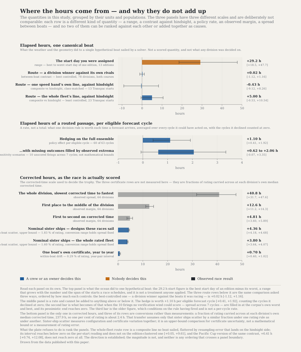
The paper reports departure-day ranges, route comparisons, forecast-policy means and corrected-time outcomes. They answer related questions but cannot be added or ranked as estimates of one effect. Table 1 names each quantity, population and comparator.
Table 1 — Where the hours come from, and what kind of quantity each one is. Grouped by unit; inside the route group, best controlled first, so that the row a reader meets first is the row the design supports best. Every route row names the corridor it was measured on. Rows may not be added together or ranked across groups. The median division in this archive finishes in 237.9 h of corrected time, so one per cent of rating is about 2.4 h.
| Lever | Hours | Interval | What kind of quantity it is |
|---|---|---|---|
| Elapsed hours, one canonical boat — not a scored quantity | |||
| The start day you were assigned | 29.2 | [18.5, 47.7] | Range: best to worst start of one edition, 13 editions (§6.4) |
| The route — a division winner against its own rivals | +0.02 | [−1.12, +1.16] | Between-boat contrast; best controlled; 78 divisions, both corridors (§5.3) |
| The route — one speed band's own line, against hindsight | −0.43 | [−9.12, +8.26] | Composite against hindsight, class-matched; 13 Transpac starts (§5.4) |
| The route — the whole fleet's line, against hindsight | 5.00 | [−0.53, +10.54] | Composite against hindsight; least controlled; 23 Transpac starts (§5.4) |
| Routed elapsed hours, per eligible forecast cycle — a rate | |||
| Hedging on the full ensemble | +1.10 | [+0.41, +1.92] | Policy effect per eligible cycle, declines scored zero, 60 of 63 (§7.1) |
| …with missing outcomes filled by observed worst and best cases | +0.62 … +2.06 | [−0.07, +3.35] | Sensitivity scenarios, not mathematical bounds; pessimistic interval reaches zero (§7.1) |
| Corrected hours, as the race is scored | |||
| The whole division, slowest corrected time to fastest | 40.8 | [31.7, 47.6] | Observed spread, 64 divisions (§6.1) |
| Winning your division rather than sitting in the middle of it | 12.6 | [11.2, 14.3] | Observed margin, first place to the division median (§6.1) |
| The margin you have to beat — first to second on corrected time | 4.81 | [3.60, 5.89] | Observed margin, 64 divisions (§6.1) |
| The certificate — nominal sister ships, race-relevant designs | 4.36 | [4.18, 4.68] | Configuration-plus-certificate scatter (§6.3) |
| The certificate — nominal sister ships, the whole rated fleet | 3.80 | [3.64, 4.07] | Configuration-plus-certificate scatter (§6.3) |
| Your own certificate's drift, de-trended, year to year | 0.70 | [0.40, 1.02] | Within-boat drift; 0.29 % of rating, converted (§6.3) |
Read across, not down. The division-level route comparison controls the most; the whole-fleet composite against hindsight controls the least. These rows answer different questions and are not additive.
1.3 How the investigation proceeds
We first hold boat, course and solver fixed while weather changes. We then introduce tracked fleets, forecast ensembles, corrected-time results and certificates. The routing results use a hypothetical boat and the fleet comparisons are observational; neither identifies why a real boat won.
Reading this paper
The paper keeps sailing vocabulary where it is useful. These are the few conversions and distinctions needed throughout.
Useful conversions
- 1° latitude = 60 nautical miles.
- 1 hour ≈ 8.9 nm for the reference boat across the historical solves.
- 1 % of rating ≈ 2.4 corrected hours on the reference passage under time-on-time scoring.
- 1 hPa ≈ 84 nm across the measured southern flank of the High; this is not a universal conversion.
Reading results
A 95 % confidence interval gives the values compatible with the data and stated procedure. If it includes zero, the sign is not established. The paper names the sampled unit—boat, division, start, edition or forecast cycle—because cases sharing weather are related. A range such as the best-to-worst start day is not an average effect. Filling missing outcomes with observed extremes is a sensitivity analysis, not a guaranteed bound. Correlation and other observational comparisons do not establish cause.
Essential terms
- Corrected time: elapsed time adjusted by the rating; it ranks boats within a division.
- Polar: boat speed by true wind angle and speed.
- Canonical boat: the hypothetical 50-footer used to hold performance fixed.
- Hindsight optimum: the solver's best route using weather that had already occurred; it was not available before the race.
- Fleet or division median line: median track latitude at each meridian; a smooth composite, not a boat's route.
- Verification replay: flying fixed geometry through verifying weather to calculate elapsed time.
- Resampling error: error introduced when geometries are placed on a shared meridian grid.
- Route separation: candidate routes remain beyond a declared threshold through 150°W; this does not establish irreversibility.
- Ensemble hedge: choosing among forecast-generated routes for performance across ensemble outcomes rather than the deterministic forecast alone.
- Route pressure: pressure sampled beneath a route; a description of where it went, not automatically a steering rule.
- Current assist: modeled current projected along and integrated over a track.
Elapsed-time replays, corrected-time results, forecast-cycle effects, departure-day ranges and certificate scatter retain their own populations and denominators.
2. Data
2.1 ERA5 as historical and verifying weather
ERA5 supplies the historical wind and the independent verification field (Hersbach et al., 2020). We use hourly 0.25° fields from the ARCO-ERA5 store (Carver & Merose, 2023). The pre-1979 back-extension is weakly constrained over the open Pacific, so it provides context only; trends begin in 1979. The most recent forecast verifications may use preliminary ERA5T, and unavailable arrivals remain unscored rather than imputed.
2.2 The ECMWF ensemble
The modern forecast experiment uses ECMWF's fifty-member IFS ensemble and the separate deterministic HRES forecast (Molteni et al., 1996; Leutbecher & Palmer, 2008). Only 00z and 12z cycles extend far enough for the passage. Member data begin in 2024. Each cycle is reduced at K = 5 and K = 8 from the same distance matrix, so the forecast cycle, not either record, is the unit of information.
2.3 The Yellowbrick fleet archive
Observed tracks cover eight Transpacs from 2011–2025 and five Pacific Cups from 2016–2026. Only boats in scored racing divisions enter fleet comparisons; retirees and non-competitive cruising or transport classes are excluded. Starts follow the actual staggered guns and therefore contain different speed bands.
Tracker fixes are sparse enough that distance is a chorded lower bound. Distance comparisons are therefore made within a division and edition. A fleet median line is a smooth composite, not a boat's track, and is not used as the rival geometry in the winner comparison.
2.4 Race results and corrected time
Division winners are identified on corrected time. Published division results are used where available; six Transpac 2015 divisions use a coefficient reconstruction and are also tested by exclusion. Time-on-time coefficients and time-on-distance allowances remain separate because they have different units. Rating-band analyses require at least five scored boats and nonzero rating spread, so one-design divisions do not enter.
2.5 ORC certificates
The certificate comparison uses public ORC records from 2019–2025 and GPH, a seconds-per-mile summary of predicted performance (Offshore Racing Congress, 2026). Sister ships are matched within rating year by design, designer, builder, length and displacement. Repeated sail numbers estimate change within one boat after removing the fleet-wide shift for each year pair.
ORC is not the rating system used by these races. Converting a fractional ORC spread to corrected-time hours assumes comparable fractional scatter under ORR and Pacific Cup rules; the race-relevant design subset checks composition, not that assumption.
2.6 Surface current
Most solves use wind and land only. HYCOM total surface current is used to separate distance through water from distance over ground and for a current-aware sensitivity on one start per edition (Chassignet et al., 2007). Comparisons stay within editions because the archive spans several HYCOM products. An altimetry-derived geostrophic field provides a lower-current cross-check (Taburet et al., 2019). These are modeled fields, not current observations beside each boat.
3. Methods
3.1 Route search
Every experiment uses the same marine isochrone search for minimum elapsed time in time-varying wind (James, 1957; Hagiwara & Spaans, 1987). Headings are spaced 2°, time steps are 20 minutes, the frontier is limited to 3,072 states, and dominance cells are 1.875 nm on a 0.25° weather grid. Frontier truncation makes the result an approximate optimum rather than proof of the global minimum.
The standard environment includes wind and land. Flat-water polars omit waves, squalls and leeway, and most solves omit current. Those omissions affect route realism and do not have a demonstrated common sign.
3.2 Canonical boat and polar panels
A hypothetical 50-foot offshore racer holds boat performance fixed while weather changes. Its elapsed time is not a published race result. Sensitivity tests use eleven Transpac polars and six Pacific Cup polars, including library and ORC-derived boats. They share starts, weather and solver settings and are therefore sensitivity cases, not independent replications.
3.3 Courses, tracks and the meridian grid
Courses use the published start and finish geometry. Route latitude is sampled where each geometry crosses a common meridian grid. Fleet lines take the median latitude of eligible boats at each meridian; they are composites and may not be continuous sailed routes.
Elapsed-time comparisons replay geometry through verifying weather. Re-cutting routes onto the grid introduces discretization error, especially for a solved optimum. Latitude and over-ground distance do not use this replay.
3.4 Ensemble candidates
The fifty member-optimal routes are partitioned by routing-outcome distance with k-medoids. K = 5 and K = 8 retain actual member routes as candidates; deterministic HRES is added to each set. Every candidate is then evaluated across all fifty members, so K limits route choice rather than the weather scenarios used for scoring.
3.5 Hedged selection
For each member, candidate regret is elapsed time above that member's fastest candidate. The hedge chooses the route with the lowest mean regret in the worst one-third of member outcomes, provided its deterministic forecast time is within 3 % of the fastest candidate (Rockafellar & Uryasev, 2000). HRES remains a normal candidate. Selecting it is a decline and contributes zero to policy gain.
3.6 Verification
ERA5 replays both the deterministic and selected routes. Gain is deterministic elapsed time minus selected elapsed time in ERA5. A firing is scoreable only when the verification field and candidate arrival window permit the comparison. Missing firings remain missing; sensitivity scenarios replace them with observed extremes or zero. Inference averages K = 5 and K = 8 within cycles and resamples calendar blocks so nearby forecasts move together.
3.7 Effect sizes and uncertainty
Inference follows the sampled unit: division for winner comparisons, start or edition for fleet comparisons, and forecast cycle for the hedge. Division results are also clustered by edition because boats in one year share weather. Estimates carry confidence intervals; null results are described as not detected rather than absent. Declared families of related diagnostics use multiplicity correction, while repeated meridians are treated as correlated descriptions rather than independent samples.
3.8 Winners against their divisions
Each corrected-time winner is compared only with boats in its own division and start. Rival tracks are resampled and replayed individually on the same canonical polar through the same weather; the comparator is the median of those individual results. This avoids treating the smoother division-median line as a boat. Retirees and tracks covering less than 80 % of the course are excluded from distance and elapsed-time comparisons.
3.9 Route separation
At each meridian, route spread is the north–south width of the complete candidate set. The separation point is the first westward crossing after which spread stays above a declared threshold through the scan ending at 150°W. The analysis sweeps 15, 30 and 60 nm thresholds and alternate grid/scan settings.
This is sustained geometric separation within the scan. It does not measure switching cost, replanning regret or irreversibility, and the finish funnel is deliberately excluded.
3.10 Converting ratings and hours
Under time-on-time scoring, corrected time is elapsed time multiplied by the coefficient, so a 0.001 change moves corrected time by one thousandth of elapsed time. Under time-on-distance, one second per mile changes corrected time by course distance in seconds. The units are never averaged.
A fractional GPH difference can be expressed as the same fractional corrected-time difference, with sign reversed, but transferring it between rating systems assumes comparable fractional scatter. Certificate hour ranges vary reference-passage duration while holding the scatter estimate fixed; they are not joint uncertainty intervals. A rating difference also represents intended performance differences, not free time.
3.11 Pressure along a route
Mean sea-level pressure is interpolated at each route crossing and time. Ridge latitude is the pressure maximum on the meridian. Candidate isobar latitude always uses the southern-flank crossing, preventing the route itself from choosing which side of the ridge counts. Fleet lines use their median clock; tracked winners use tracker time; forecast routes are replayed in the verifying field.
3.12 Distance through water and current-aware routing
For each tracker leg, ground displacement is combined with modeled current at the leg's midpoint to estimate water displacement and current assist. Sparse legs are subdivided before sampling rather than discarded. Alternative lanes are integrated at a common fleet pace. One start per edition is solved both with and without current to test how the modeled field changes the optimum and the fleet comparison.
The current-aware solver adds current to speed over ground but does not solve a separate cross-track heading correction. The same approximation is applied to both routes in the sensitivity comparison.
4. The ocean: the route trade and where alternatives separate
4.1 From advice to measurements
Transpac guides describe the same ridge-crossing problem: the shorter northern line approaches the light air under the High, while sailing south usually adds distance and wind. We first measure where plausible routes separate, then hold the boat fixed and change its July departure. Latitude describes the geometry; pressure connects it to the weather chart.
4.2 Where the routes stop reconverging
Route separation is the first meridian after which the north–south spread of a route set stays above a declared threshold through 150°W. Routes that split and rejoin before that boundary do not count. The measurement says nothing about later reconvergence, switching cost or irreversibility.
The forecast family contains the ensemble cluster representatives plus deterministic HRES. The historical comparison asks where one July's hindsight optimum leaves the long-run average line and remains separate through the same boundary. The forecast cycle is the unit; K = 5 and K = 8 are two clusterings of each cycle, not independent samples.
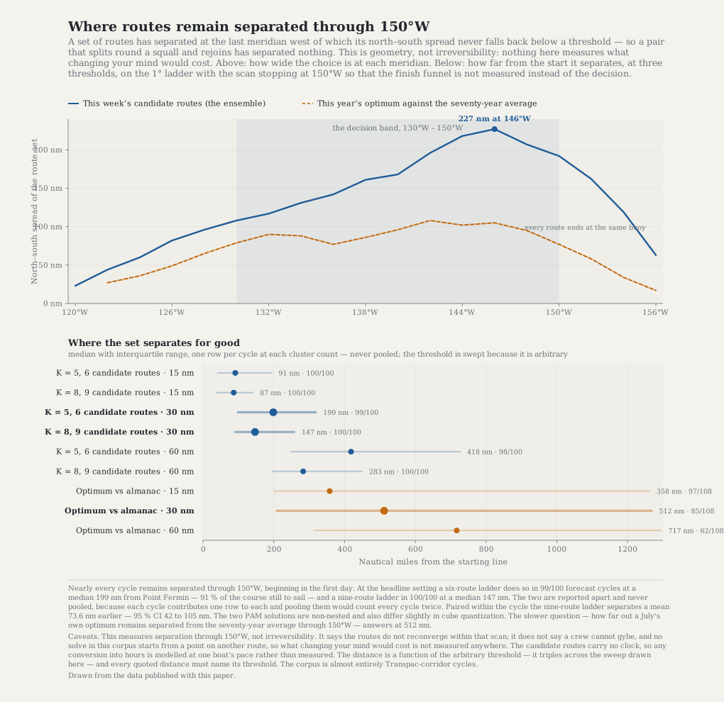
Move the threshold and compare K = 5 with K = 8. Notice both how early the route set separates and how much the answer depends on the threshold.
Table 2 — First sustained separation through 150°W. The headline uses a 30 nm threshold and 1° meridian grid. Distance is measured from the start along the set's median line.
| Route family | Separated | Median distance from start |
|---|---|---|
| Candidates, six routes (K = 5) | 99/100 | 199 nm |
| Candidates, nine routes (K = 8) | 100/100 | 147 nm |
| Hindsight optimum against the almanac line | 85/108 | 512 nm |
The candidate routes usually establish sustained separation during the first day. K = 8 separates earlier than K = 5, but the medoids are not nested, so this is not an experiment in candidate count. At a 15 nm threshold the medians are about 90 nm; at 60 nm they are 418 and 283 nm. The exact distance is a property of the declared threshold. The supported result is simply that substantial alternatives form early and remain separate through 150°W.
4.3 What five days does to the same boat
Hold the canonical boat, course and solver fixed. Route it through each year's ERA5 weather from 6, 11 and 16 July, then compare departures within the same year and fitted change across years.
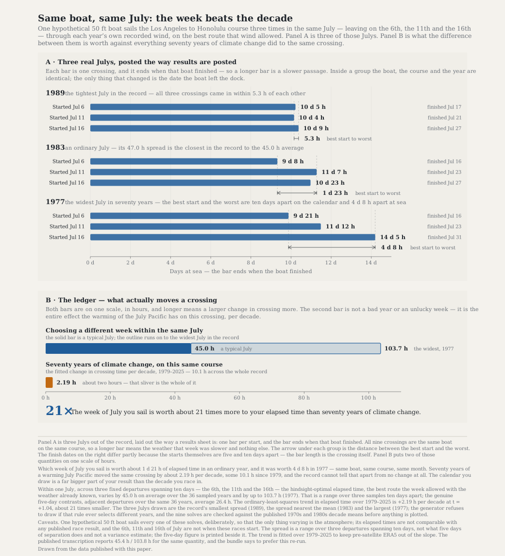
Move the departure from 6 to 11 to 16 July. The route and elapsed time change even though the boat and course do not.
Table 3 — Variation against fitted change, 1979–2025. The all-solve spread includes variation within July; the year-mean spread describes differences between Julys.
| Quantity | Spread across all solves | Spread of year means | Fitted change across record |
|---|---|---|---|
| Optimal elapsed time | 24.7 h | 14.5 h | 10.1 h |
| Route latitude at 142°W | 2.19° | 1.5° | 0.50° |
Adjacent departures five days apart differ by 26.4 h on average. Across all three dates, the best-to-worst ten-day range averages 45.0 h. These are different statistics: 26.4 h describes two boats leaving five days apart; 45.0 h describes the span of the sampled July window.
Across 1979–2025, no trend is detected in optimal elapsed time, distance, maximum latitude or route latitude at the declared meridians. The fitted elapsed-time change is +10.1 h [−9, +29]; at 142°W the fitted latitude change is +0.50° [−1.2°, +2.2°]. The intervals still admit changes that could matter. The result is “no drift detected,” not “no drift occurred.”
Figure 4 shows the complete route archive and the fitted latitude lines.
Scroll horizontally to inspect the chart labels.
Figure 4 — The optimum through seventy years. The top panel is a chart of the North Pacific with every one of the 108 solved routes drawn on it — three July departures in every odd year from 1955 to 2025 — and the heavy line through them is their mean lane. The dashed straight line is the rhumb line from Point Fermin to Diamond Head, the two dotted meridians are the lines of longitude the study reads each route at, and the bracket on each is that meridian’s ±1 sd put back on the water. Below, one panel per meridian: each dot is one departure’s latitude there, the vertical bars join the three departures of a single July, and the straight line is the trend fitted over the satellite era. Up the page is north throughout. The flat-water, wind-and-land-only hindsight optimum was solved with each year’s weather already known. The whole seventy-year bundle lies in one band about four hundred miles deep, and the fitted line is flat at both meridians. The experiment detected no trend, but its interval still admits passage-scale changes that could matter: across the satellite era the fitted change in elapsed time is +10 h on a 95 % interval of [-9, +29] h. What the route does instead is jump around, and the three departures inside one July are often further apart than the whole fitted change across the record. Points before 1979 are drawn but never fitted, because ERA5 has no satellites to work with that far back.
Evidence and limits
- 134°W: year-to-year sd 1.91° — 115 nm — trend +0.012°/decade (t = +0.07).
- 142°W: year-to-year sd 2.19° — 131 nm — trend +0.108°/decade (t = +0.58).
- The three departures within one July routinely differ by more than the whole fitted change across 47 years.
- The chart panel is Mercator, so the rhumb line is straight and a degree of latitude is sixty miles anywhere up the page; the scale bar names the latitude its miles are true at, because on Mercator east–west scale grows northward. Coastline: Natural Earth 1:10m, clipped to the corridor and committed with the rest of the data.
- The canonical boat is nobody's boat, and its elapsed times are not comparable with any published race result.
- The lower panels read latitude on a 4° meridian ladder, and the departures are three fixed calendar dates rather than a real race start.
- The chart draws each route from the pressure sweep’s one-degree crossings, which begin at 122°W: the first two hundred miles out of Point Fermin are not on the plate. The two files are the same 108 solves, and the figure refuses to draw unless their shared ladder readings agree to a thousandth of a degree.
- The published transcription
optimum-historical.json(Prototype B, 109 solves) differs slightly from this re-run; the bundle says to prefer the re-run, and this figure plots it.
The canonical boat is not a historical competitor, the dates are not assigned race starts, and three-hourly weather smooths shorter-lived conditions.
4.4 The same decision, read as pressure
A navigator sees the High as a ridge and its surrounding isobars. That suggests a self-adjusting rule: use a target pressure on the ridge's southern flank rather than a fixed latitude. Route pressure is the median mean-sea-level pressure beneath a route while it crosses 130–150°W.
This pressure rule is a hypothesis tested here, not published race advice. The optimum's median route pressure is 1021.5 hPa, and no trend is detected. A stable description, however, is useful for navigation only if it predicts the lane better than latitude.
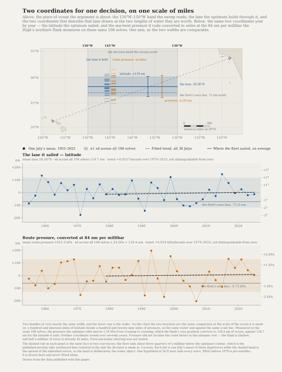
Toggle the same solved route between latitude and pressure. The route does not move; only its coordinate changes. Then compare the rules out of sample.
Table 4 — Latitude and pressure almanacs scored against the same unseen Julys. The pressure rule learns a target from earlier years and is shown the current year's analysed pressure chart.
| Rule | Julys | MAE | RMSE |
|---|---|---|---|
| Latitude almanac | 30 | 60.3 nm | 77.3 nm |
| Isobar almanac | 30 | 98.5 nm | 117.6 nm |
Pressure is not the better almanac. Its RMSE is 40 nm larger even though it receives the year's chart. The physical reason is the shallow southern flank: across these routes, 1 hPa corresponds to about 84 nm of latitude. A half-millibar difference is already about 42 miles.
Pressure remains useful for describing the weather around a route. This experiment uses reanalysis and does not test whether a navigator can forecast or steer a target isobar six days ahead.
4.5 Why a seasonal mean cannot locate one start
A seasonal mean can describe the kind of July but not the weather of a particular departure. Most of the elapsed-time variation in this experiment occurs within July rather than between year means. Even a perfect prediction of the summer average would not tell a navigator whether the 6th, 11th or 16th contains the faster crossing.
5. The fleet: what winners actually do
5.1 How the fleet and hindsight are compared
Section 4 held the boat fixed. We now add real fleets and ask two questions: do they move with the best route at the year and start scales, and what distinguishes a division winner from the boats it actually beat?
The Yellowbrick archive covers eight Transpacs, 2011–2025 (435 boats in 23 starts), and five Pacific Cups, 2016–2026 (259 boats in 18 starts). At the start level, each fleet is compared with the canonical boat's hindsight optimum for its own gun. At the division level, 78 divisions across twelve editions have at least five tracked boats and an identifiable corrected-time winner.
The comparison replays four geometries through the same weather: the fleet-median line, a static line formed from all editions, the rhumb line and individual tracked boats. Prior work makes related track-to-route comparisons inshore (Forsberg et al., 2024) and in the Southern Ocean (Goto et al., 2024).
Everything in this section lives inside the routing-software era: coverage begins in 2011 and 2016, and nothing here says what a 1985 fleet would have done.
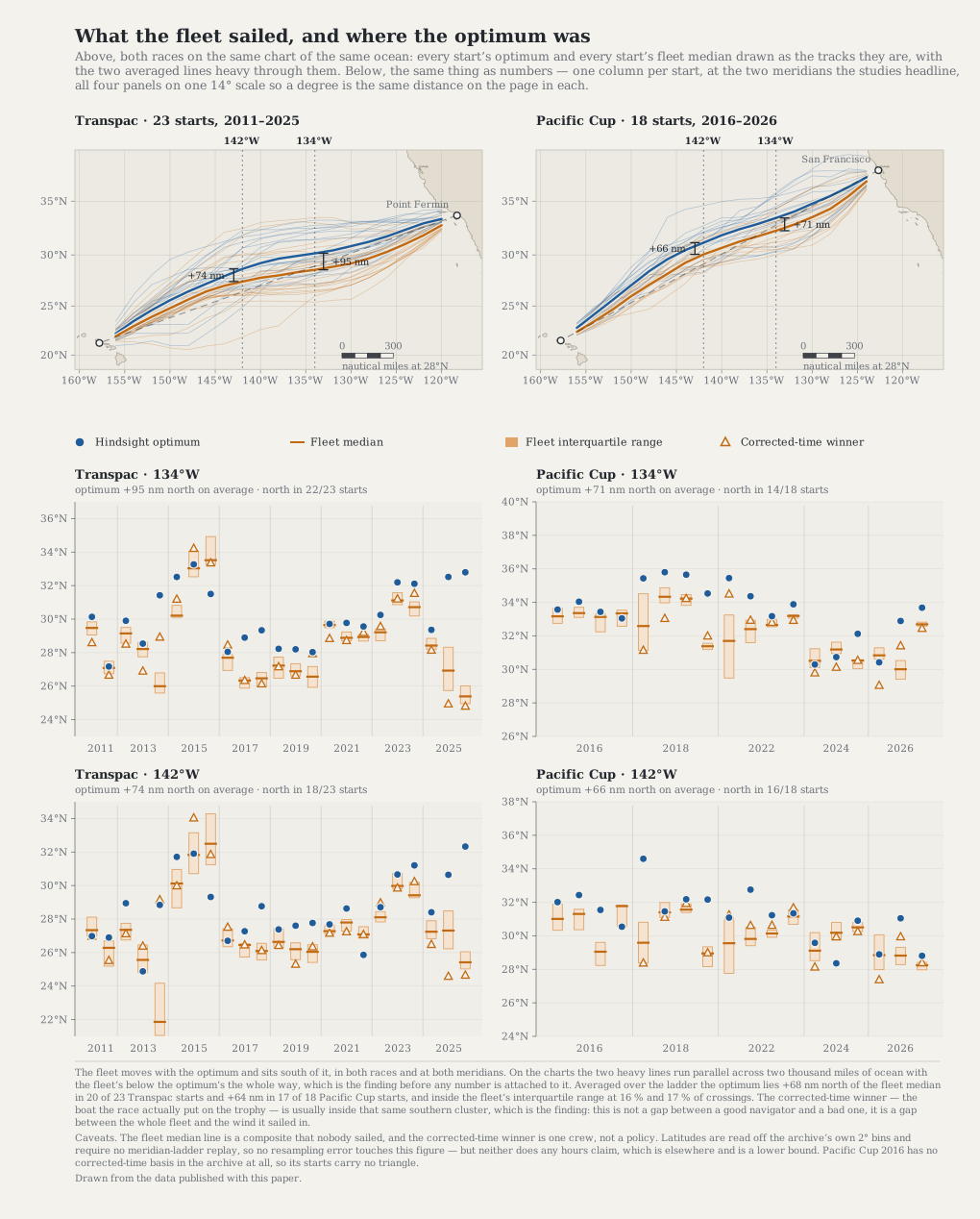
Figure 6 draws both races on one chart, every start's optimum against its fleet-median line, and then the same latitudes as numbers with each start's interquartile band and its corrected-time winner.
Scroll horizontally to inspect the chart labels.
Figure 6 — What the fleet sailed, and where the optimum was. The two charts are the same ocean at the same scale, one race each: every thin blue line is one start’s hindsight optimum and every thin orange line is that start’s fleet median, with the average of each drawn heavy through them, and the bracket on each dotted meridian is the gap between those two averages in miles. Below, four panels — two races by two meridians. Every column is one start: the dot is the optimum’s latitude there, the band is the middle half of that start’s fleet with its median, and the triangle is the start’s corrected-time winner. Up is north throughout, and the columns are grouped by edition. In both races and at both meridians the fleet swings the same way the perfect route swings from one year to the next — and sits south of it almost every time, by roughly a degree of latitude, sixty miles. On the chart that gap is two lines running parallel across the whole ocean, one of them a scale-bar’s width below the other. The boat that won on handicap is usually inside that same southern cluster, so this is a whole-fleet pattern rather than a story about good and bad navigators.
Evidence and limits
- Transpac at 134°W: optimum a mean +95 nm north of the fleet median, north in 22 of 23 starts.
- Transpac at 142°W: optimum a mean +74 nm north of the fleet median, north in 18 of 23 starts.
- Pacific Cup at 134°W: optimum a mean +71 nm north of the fleet median, north in 14 of 18 starts.
- Pacific Cup at 142°W: optimum a mean +66 nm north of the fleet median, north in 16 of 18 starts.
- The chart panel is Mercator, so the rhumb line is straight and a degree of latitude is sixty miles anywhere up the page; the scale bar names the latitude its miles are true at, because on Mercator east–west scale grows northward. Coastline: Natural Earth 1:10m, clipped to the corridor and committed with the rest of the data.
- The fleet median line is nobody's track, and it is shorter than any of them.
- A corrected time is one of three bases, and the archive cannot always support one.
- Nothing in the panel is a multihull.
- Some of the offset comes from the comparison rather than the fleet: a hindsight optimum can shave the light air under the ridge using information a forecast-bound navigator lacks, and the optimiser sees wind and land but no sea state.
- No hours claim appears here. Latitudes are read off the archive’s own 2° bins and require no meridian-ladder replay, so resampling error does not affect this figure.
5.2 Fleets read the year, and not the week
Real fleets move with the year on both courses; they do not follow a fixed remembered line.
Across editions, the fleet's median latitude and the optimum's are positively correlated at every one of Transpac's 19 meridians, from r = +0.673 at 138°W to r = +0.945 at 154°W (n = 8 editions). The Pacific Cup shows the same direction: r = +0.911 at 124°W and +0.877 at 134°W across five editions. Edition is the primary unit because starts within an edition share weather. With only eight and five editions and strongly correlated adjacent meridians, the direction is clearer than the exact size of the association.
Start-to-start changes do not track the optimum
Each edition contains a partly-controlled experiment the years cannot provide: divisions starting one to four days apart, and up to five days end to end on Transpac, sailing into materially different weather with one fleet's culture and one season's knowledge. These starts do not contain the same boats: both races stagger their starts by speed, so on Transpac the first start's modal class is a J/122 or a Cal 40, the second's a Santa Cruz 50 and the third's a Santa Cruz 70. The starts group divisions by speed, and that stratification uses the kind of averaged handicap number §2.5 describes.
That matters because of what it does to the measurement. A canonical-boat comparison correlates each fleet's start-to-start latitude shift with an optimum flown on one 50-foot polar at every gun. The fleet's shift therefore contains a boat-type term the optimum's cannot contain by construction, and an additive term present in one variable and absent from the other attenuates a correlation toward zero. The matched comparison instead flies each start's optimum on the panel polar selected by its division band.
Table 5 — Start-to-start fleet shifts against canonical and division-matched optima. 22 unordered start pairs on Transpac, 24 on the Pacific Cup.
| Corridor | Meridian | Canonical 50-footer | Polar-matched | 95 % CI | p |
|---|---|---|---|---|---|
| Transpac | 134°W | −0.203 | +0.048 | [−0.38, +0.46] | 0.831 |
| Transpac | 142°W | −0.157 | −0.108 | [−0.51, +0.33] | 0.631 |
| Pacific Cup | 134°W | +0.233 | +0.334 | [−0.08, +0.65] | 0.110 |
| Pacific Cup | 142°W | −0.177 | +0.198 | [−0.22, +0.56] | 0.353 |
Polar matching removes the negative pattern in the canonical comparison, and every interval in Table 5 includes zero. The fleets still move about as far between starts as the optimum does, but their direction has no detected relationship with the optimum's. The year-scale association is stronger.
With 22 and 24 start pairs, correlations of roughly ±0.4 remain compatible with the data. The supported statement is “no detectable start-scale signal,” not “independence.”
5.3 What the boat that won its division actually did
The fleet-median comparisons above answer "where was the middle of the fleet". They cannot answer the question an owner asks, which is what the boat that won the trophy did differently from the boats it beat. That needs the division as the unit and the division's own boats as the control, which is the construction of §3.8. Seventy-eight divisions over twelve editions qualify — 50 Transpac, 28 Pacific Cup.
Table 6 — What the winner did, against the boats it beat. Every quantity is the corrected-time winner of a division measured against the median of that division's own boats.
| Quantity | n | Mean [95 % CI] | Median | Sign test |
|---|---|---|---|---|
| Distance over the ground, winner minus its rivals' median | 78 | −12.0 nm [−22.6, −1.5] | −6.1 | 25/74 longer, p = 0.007 |
| Distance through the water, the same construction | 78 | −10.7 nm [−20.6, −0.8] | −9.0 | 28/72, p = 0.076 |
| The current the winner was given, minus its rivals' | 78 | −0.72 nm [−3.77, +2.33] | +0.27 | 40/78, p = 0.910 |
| Latitude, winner minus its division's median, north positive | 78 | −0.5 nm [−11.1, +10.2] | +2.5 | 43/78, p = 0.428 |
| Closeness to the optimum, winner minus its rivals | 78 | −2.4 nm [−9.6, +4.8] | 0.0 | 36/73, p = 1.000 |
| Elapsed hours, winner minus its rivals, 1° grid | 78 | +0.02 h [−1.12, +1.16] | — | — |
Winners were not detectably north or south of their rivals, and they were not detectably closer to the hindsight optimum. The latitude difference was −0.5 nm [−11.1, +10.2]; the closeness difference was −2.4 nm [−9.6, +4.8].
Their recorded tracks were shorter more often than not: −12.0 nm over the ground [−22.6, −1.5] and 0.02 h in the replay comparison [−1.12, +1.16]. Re-cutting the tracks onto a meridian grid removes the distance difference because the grid retains strategic latitude but discards gybes, squall dodges and smaller steering changes. A composite median line is also artificially smooth, so it is not a valid substitute for replaying each rival's track individually.
This is observational. Divisions share weather within an edition, tracker cadence cannot resolve the manoeuvres behind the distance difference, and a shorter track may be a consequence of being in phase with the weather rather than its cause. The association does not establish why winners sailed less distance.
No systematic current-assist difference is detected. After correcting each track with the same ocean-current model, winners sailed 10.7 nm less through the water than their rivals [−20.6, −0.8]. The current-assist difference itself was −0.72 nm [−3.77, +2.33]. Boats within the same division nevertheless differed by a mean 29.6 nm from the best-served to the worst-served. Current mattered within races, but this analysis detected no systematic current advantage for the winner. The correction uses modeled surface current rather than direct observations, so its magnitude remains uncertain.
Six of the 78 divisions, all from Transpac 2015, use the weakest corrected-time reconstruction. Excluding them does not change the result.
Distance and corrected finishing place
The whole-division association points in the same direction. Inside a division, boats that sailed farther over the ground tended to finish worse: Spearman ρ = +0.239 on Transpac, +0.194 on the Pacific Cup and +0.221 pooled across 72 divisions. The pooled association is about half the +0.40 measured in the Chicago–Mackinac study.
Course geometry may contribute to the weaker association. The Chicago–Mackinac course is under 300 nm and almost all of it is avoidable wandering. A 2 220 nm ocean crossing is mostly a straight line down the trades, so a much smaller fraction of the total distance is discretionary. That can attenuate the correlation.
The comparison is observational. Nobody assigned a division a route. A winner's shorter track could be the cause of the win, a consequence of better sailing that the tracker also records as less wandering, or a consequence of that boat having been in phase with the weather it was given.
5.4 From the observed offset to elapsed time
Winners and fleets both sail south of the wind-only hindsight optimum.
At the division level, the winner's line sits 88.5 nm south of its own start's flat-water, wind-and-land-only hindsight optimum [−114.6, −62.4]. Its division's median line sits 88.0 nm south [−112.6, −63.5]. At the start level, the optimum is also north of the fleet median on both courses.
Table 7 — The northward offset of the optimum from the fleet median. Positive is north.
| Corridor | Per start | Per edition |
|---|---|---|
| Transpac | +67.9 nm, n = 23, CI [+32, +104] | +66.7 nm, n = 8, CI [+23, +110] |
| Pacific Cup | +62.4 nm, n = 18, CI [+35, +90] | +61.1 nm, n = 5, CI [+20, +102] |
This is not evidence that the fleet made a navigational error. The optimizer knew the weather that followed; the navigators did not. Sailing south is consistent with avoiding the light-air failure mode under the High, but the archive does not measure crews' risk preferences. Flat-water polars, omitted sea state, squalls, crew performance and boat mismatch can also contribute. The design cannot apportion them.
One forecast comparison supports the direction without establishing the cause. Against the 2025 Transpac fleet, the deterministic route sits 88 nm north of the fleet median; the ensemble hedge moves south to 59 nm. That is one edition, not an explanation of the historical fleet offset.
The southern lane also receives slightly more favourable modeled current in this sample. The optimum's lane collects 6.4 nm less free distance [3.6, 9.2], about 0.8 h at the fleet's speed. This cannot be combined with the whole-fleet +5.00 h contrast or the winner-versus-rivals +0.02 h contrast because they use different populations and comparators.
Three comparisons of elapsed time
Elapsed-hour comparisons are sensitive to replay and resampling error, so each is reported with its construction and uncertainty. There is a second reason for care here, and it matters more than the first. This study can compare a fleet's route against a better route in three different ways, and the three control for very different amounts. They are different estimands and cannot be averaged or differenced. We construct them from the most controlled population outward.
Start with one division winner and the boats it raced. Then widen the comparator to a speed-band median and finally the whole fleet. Each step replaces real boats and shared conditions with a broader composite or hindsight benchmark.
Best controlled — the division winner against its own rivals. Each tracked boat is replayed individually on the same canonical polar through the same weather. Across 78 divisions in 12 editions, the winner-minus-rivals estimate is +0.02 h [−1.12, +1.16] using divisions and +0.02 h [−1.09, +1.13] when editions are resampled. The mean is near zero. This constrains route geometry; it does not say that navigation has no effect.
Partly controlled — a fifty-footer against its class line. The canonical polar flies the median line of the archive's 50-foot band and that start's hindsight optimum. Across 13 Transpac starts in eight editions, the estimate is −0.43 h [−9.12, +8.26]; the edition-resampled interval is [−8.05, +6.37]. The interval is too wide to resolve the difference, and the class line remains a composite.
Least controlled — the whole-fleet line against hindsight. On Transpac, the canonical polar flies the whole fleet's median line and the hindsight optimum. Across 23 starts in eight editions, the difference is +5.00 h. The start-level interval is [−0.53, +10.54]; the edition-resampled interval is [+0.05, +9.61]. The procedures disagree about whether the interval clears zero. On the Pacific Cup, the corresponding estimate is +6.41 h [+0.74, +12.08]. The direction is mostly consistent across starts, but this is the least controlled comparison.
The three numbers are not successive measurements of one effect. The winner comparison pools divisions from both races; the other two use Transpac starts. Their units, populations and comparators differ.
The whole-fleet comparison has biases as large as its estimate. The median line is a smooth composite that nobody sailed, it mixes boats of different speeds, and resampling adds +7.4 h [3.16, 11.64] to the replayed optimum. Matching the canonical boat to its class collapses the contrast toward zero. The wind-only whole-fleet estimate has not been validated under current.
The supported statement is narrow: the fleet median line was usually slower than the hindsight optimum, but the magnitude is unresolved and cannot be interpreted as five hours available to a navigator.
5.5 What §5 does not establish
These comparisons are observational. They show what winners and fleets did, not what caused them to win or why they chose a lane. The division, class-band and whole-fleet comparisons use different populations, units and comparators, so they cannot be averaged or differenced as estimates of one effect. Latitude and distance come directly from track geometry; elapsed-hour comparisons also carry verification-replay and resampling error.
6. Ratings, start dates and the boat
Sections 4 and 5 isolate weather and route choice. Corrected-time results also depend on the scoring rule, the certificate, the assigned start and the boat whose polar goes into the router. This section puts those quantities into hours where the conversion is defensible, while keeping unlike measurements separate.
Common units let us compare the scale of these quantities. They do not make the underlying estimands equivalent.
6.1 How much corrected time does a rating point move?
A boat's rating is the number used to adjust elapsed time. The adjusted result is corrected time, which determines the winner. Under time-on-time scoring, corrected time is elapsed time multiplied by a coefficient. Changing that coefficient by 0.001 therefore changes corrected time by one thousandth of the elapsed time. Section 3.10 gives the arithmetic and §2.4 explains how we identified each division's scoring regime.
Fifty-eight divisions across nine editions use time-on-time scoring. Six divisions, all from Transpac 2011, use time-on-distance. The first group contains 397 boats and the second 36. A thousandth of a coefficient and a second per mile are different units, so we never average them.
Table 8 — What a rating point is worth, and what it has to beat. Medians across divisions with 95 % intervals. Converted rows are marked with a dagger.
| Quantity | Median | 95 % CI |
|---|---|---|
| Price of 0.001 of a time-correction coefficient | 0.267 h | [0.238, 0.285] |
| The rating change that would have flipped the division win | 19.0 | [14.9, 26.4] |
| † The whole fleet's route deficit, expressed as rating | 18.7 | [−2.0, +40.6] |
| † The hedge, expressed as rating | 4.12 | [+1.6, +7.4] |
| First to second on corrected time | 4.81 h | [3.60, 5.89] |
| First to the division median | 12.6 h | [11.2, 14.3] |
A thousandth of coefficient is worth a median 0.267 h. First and second finish 4.81 h apart, and 19.0 thousandths would flip the median division result. The whole-fleet route contrast converts to 18.7 thousandths [−2.0, +40.6]; the ensemble hedge converts to 4.12 [+1.6, +7.4]. The route interval crosses zero, so the similarity between 19.0 and 18.7 does not establish equal importance.
These conversions put quantities on a common scale; they do not make them the same estimand. A lower rating is also intended to compensate for lower boat speed, so rating is not free elapsed time.
6.2 Where do winners sit in the rating band?
The familiar claim is that a boat should sit near the slow-rated end of its division, especially in a light year. We can test that position directly. Within each division we rank boats by rating after fixing the sign so that a larger value always means a faster-rated boat. The winner's percentile is 0 for the slowest-rated boat and 1 for the fastest; ties take the midrank. Divisions with fewer than five scored boats or no rating spread are excluded. One-design classes such as the Cal 40 division therefore do not enter this comparison.
Table 9 — Where the corrected-time winner sits in its division's rating band. 0 is the slowest-rated boat in the class, 1 the fastest.
| Sample | n | Median percentile | 95 % CI | Test |
|---|---|---|---|---|
| All divisions | 64 | 0.500 | [0.375, 0.600] | sign 29/57, p = 1.00 |
| Clustered — one median per edition | 10 | 0.533 | [0.367, 0.775] | sign 5/9, p = 1.00 |
| Light-weather starts | 33 | 0.400 | [0.250, 0.600] | — |
| Heavy-weather starts | 31 | 0.556 | [0.429, 0.800] | Mann–Whitney z = −1.54, p = 0.124 |
Across 64 divisions, the median winner is exactly halfway through its rating band: 0.500 [0.375, 0.600]. Collapsing each edition to one median gives the same result. Rating position alone does not identify an advantage.
Light-weather winners sit lower in the band than heavy-weather winners, 0.400 against 0.556, but the difference is not detected (p = 0.124). The percentile measures position rather than the absolute width of the band.
6.3 How far apart are certificates for the same hull?
Table 8 gives the corrected-time value of a rating difference. The public Offshore Racing Congress certificate archive lets us compare the size of those differences. We separate scatter between boats of the same design from year-to-year movement in one boat's certificate. The first includes legitimate configuration differences; the second removes fleet-wide changes to the rule.
Table 10 — Certificate scatter and within-boat drift. Relative spread uses GPH, the ORC General Purpose Handicap. Hour ranges use the Hawaii reference passage.
| Population | Relative spread | 95 % CI | Hours on this course |
|---|---|---|---|
| Matched sister ships | 1.60 % | [1.50, 1.69] | 3.80 h |
| Matched sister ships from designs sailed in these races | 1.83 % | [1.53, 2.24] | 4.36 h |
| One boat, year to year, after removing the fleet-wide shift | 0.29 % | [0.285, 0.300] | 0.70 h |
Switch between the sister-ship samples and repeated certificates for one boat. The first two comparisons are between boats; the third is change within a boat.
Matched sister ships differ by 1.60 % [1.50, 1.69]. Designs sailed in these races give a similar 1.83 % [1.53, 2.24]. On the reference passage those point estimates correspond to 3.80 and 4.36 hours. The hour values vary passage duration; they are not joint uncertainty intervals.
Within one boat, the typical de-trended year-to-year movement is much smaller: 0.29 % [0.285, 0.300], or about 0.70 h on the same passage. Grouping by year pair rather than boat widens the diagnostic range to 0.176–0.399 %, showing that typical movement varies between seasons.
Sister-ship scatter is not certificate error. Nominally identical hulls can differ in sails, propeller, keel, loading and displacement. The result measures configuration-plus-certificate scatter, not gaming or measurement error. Transferring the fraction from ORC to races scored under ORR and Pacific Cup rules also assumes that comparable hulls scatter similarly under those systems. The archive cannot test that assumption.
6.4 What does the start day do to the same boat?
Both races stagger divisions so boats of different speeds converge near the finish. That choice helps race management, but it also puts different divisions into different weeks of weather. We can isolate its scale without changing boat or solver: route the canonical boat with perfect knowledge from every actual gun in an edition, then compare the fastest and slowest crossing.
Table 11 — Start-day weather, edition by edition. Spread is the fastest-to-slowest hindsight result for the same boat across an edition's actual guns.
| Edition | Starts | Span (d) | Spread (h) |
|---|---|---|---|
| Pacific Cup 2016 | 4 | 4.2 | 18.5 |
| Pacific Cup 2018 | 4 | 4.1 | 34.2 |
| Pacific Cup 2022 | 4 | 4.1 | 51.7 |
| Pacific Cup 2024 | 3 | 3.1 | 47.7 |
| Pacific Cup 2026 | 3 | 4.1 | 21.2 |
| Transpac 2011 | 2 | 4.0 | 27.8 |
| Transpac 2013 | 3 | 5.0 | 37.2 |
| Transpac 2015 | 3 | 5.0 | 49.0 |
| Transpac 2017 | 3 | 3.0 | 21.0 |
| Transpac 2019 | 3 | 3.0 | 7.0 |
| Transpac 2021 | 3 | 4.0 | 6.7 |
| Transpac 2023 | 3 | 4.0 | 29.2 |
| Transpac 2025 | 3 | 4.0 | 31.3 |
Across thirteen editions, the median within-edition spread is 29.2 h [18.5, 47.7], or about seven hours per day between starts. It ranges from 6.7 h in Transpac 2021 to 51.7 h in Pacific Cup 2022. This is a fastest-to-slowest range, not an estimated effect, and it grows with the number and spacing of starts.
The same weather difference appears in results: a boat's start-specific optimum and fleet-wide corrected time have a pooled Spearman ρ = +0.450, so boats assigned slower weather tended to score worse. The comparison is observational because each start contains different boats.
Forecast-adjusted scoring is intended to reduce this unequal treatment by rating representative boats in the weather expected for each start. Transpac introduced that approach in 2025. Table 11 measures the historical weather difference before enough post-change editions exist to evaluate how much remains.
6.5 The fastest route depends on the boat
Across eleven boats, the long-run mean latitude of the optimum differs by no more than 1.5°. That aggregate hides large paired differences on individual crossings. To isolate them, we route every panel boat from the same Transpac gun through the same ERA5 cube. The only changing input is the polar. We then compare each boat's mean latitude across the decision band with the canonical 50-footer on that same crossing.
Table 12 — Where each boat's optimum runs, against the canonical 50-footer on the same crossing. Transpac, 23 crossings each. Positive is north. Reaching speed is the panel's summary of each polar.
| Polar | Reaching kt | vs the canonical boat, nm north |
|---|---|---|
| orc-alive (R/P 66) | 15.44 | −11.9 [−55.3, +31.4] |
| orc-tp52 (TP 52) | 13.84 | −4.6 [−43.1, +33.9] |
| orc-aragon (Marten 72) | 12.92 | −1.9 [−35.8, +32.0] |
| tp52 (library) | 12.33 | +7.6 [−29.9, +45.2] |
| sled70 (Santa Cruz 70) | 11.47 | +2.3 [−37.3, +41.9] |
| orc-vortices (J/125) | 11.23 | −2.7 [−22.6, +17.3] |
| sc50 (Santa Cruz 50) | 10.53 | +29.9 [+2.7, +57.1] |
| canonical 50 ft | 10.24 | — |
| orc-j121 (J/121) | 9.74 | +50.8 [+19.4, +82.2] |
| j122 (J/122) | 9.01 | +58.1 [+23.6, +92.7] |
| cal40 (Cal 40) | 7.65 | +46.2 [+1.2, +91.2] |
The slower boats' optima run north. The fastest boats remain within 12 nm of the canonical route, while the Santa Cruz 50, J/121, J/122 and Cal 40 run 29.9 to 58.1 nm north through the decision band. The panel's north–south spread reaches 114 nm at 138°W. Certificate-derived and library polars give compatible comparisons for the J/12x and TP52 pairs.
To identify which part of a polar moves the route, we perturb three separate regions by ±5 % while holding the rest fixed. The regions are upwind at 40–52° true wind angle, reaching at 75–120°, and deep running at 145–180° in 16–20 kt of true wind. The wind-speed restriction isolates running in the trades.
Table 13 — Which dimension of the canonical polar moves the route. Mean-latitude shift through the decision band against the unperturbed boat on the same 11 crossings.
| Perturbation | Factor | Shift, nm north [95 % CI] |
|---|---|---|
| downwind | ×0.95 | +25.0 [+7.6, +42.4] |
| downwind | ×1.05 | −17.6 [−33.1, −2.0] |
| reaching | ×0.95 | −5.5 [−20.1, +9.2] |
| reaching | ×1.05 | +5.0 [−1.8, +11.7] |
| upwind | ×0.95 | +2.5 [−17.7, +22.8] |
| upwind | ×1.05 | +1.7 [−2.9, +6.2] |
Figure 7 shows the six library polars, the optimum for each boat, the maximum separation among those routes and the elapsed-time cost of each comparison geometry.
Scroll horizontally to inspect the chart labels.
Figure 7 — The same ocean, six different boats. The upper panel plots where each of six boats’ optimum runs, meridian by meridian, inside a shaded envelope showing how far apart they ever get. The lower panel is hours: each group of bars is one boat, and each bar one comparison geometry — what that geometry cost that boat against its own hindsight optimum. Change the boat and the lane moves less than elapsed time, but it still moves. The six-boat panel stays inside the envelope drawn here; the eleven-boat panel reaches 114 nm of latitude separation. Latitude is less sensitive to polar than elapsed time in the six-boat panel, but it is not boat-independent.
Evidence and limits
- The panel’s widest disagreement about latitude at any meridian is 1.30° (78 nm).
- The canonical reference boat sits inside the envelope at every meridian — it is the panel median on northward bias.
- Hours given up run from −0.4 h to +18.5 h across boats and geometries: strongly boat-dependent, and not monotonic in boat size.
- The canonical boat is nobody's boat, and its elapsed times are not comparable with any published race result.
- Class-matched columns rest on 1 to 13 waves and are suggestive, not results.
- Elapsed-hour bars include meridian-ladder resampling error.
- This plate draws the six library polars. The eleven-polar envelope quoted in the text is wider than the six-boat one drawn here.
- The panel varies the boat uniformly across every start, so it is a sensitivity check on one nuisance parameter and not evidence about anything that differs between starts.
Only the deep-running perturbation moves the canonical boat's route. Reducing that speed by 5 % moves the optimum 25.0 nm north [+7.6, +42.4] and adds 6.2 h. Increasing it by 5 % moves the optimum 17.6 nm south [−33.1, −2.0] and saves 5.7 h. The upwind and reaching changes alter elapsed time but leave route latitude consistent with zero.
The paired results support a physical hypothesis: a boat that runs slowly in the trades may gain more by staying in stronger northern wind, while a faster runner can accept the shorter southern line. The experiment changes one region of one polar, so it does not establish that running speed causes the full between-boat pattern.
Boat dependence and route separation are distinct. The boat changes which route is fastest; the weather changes where candidate routes achieve sustained separation within the assessed scan.
6.6 Limits of these comparisons
The scoring units remain separate: a thousandth of a time-on-time coefficient cannot be averaged with a second per mile. Rating position is descriptive, one-design divisions have no rating band, and division results share weather within editions. Start-day comparisons cannot separate weather from the boats assigned to each gun. Sister-ship scatter combines configuration and certificate differences, and moving it from ORC to other rating rules requires an untested transfer assumption. The boat-route comparisons use one solver with wind-only physics; their proposed running-speed mechanism remains unestablished.
7. From a forecast to a route decision
The routes in §§4–6 use weather that had already happened. A navigator instead has several plausible futures and must choose a route before knowing which one will occur. This section asks whether selecting a route that performs acceptably across an ensemble improves on following the deterministic forecast alone. ERA5 verifies both routes so that the forecast does not grade itself.
7.1 One decision first, then the whole policy
For one cycle, the fifty ensemble members describe fifty possible weather evolutions. We cluster them into representative members, route the canonical boat on each medoid, and add the deterministic route. Each candidate is evaluated across the full ensemble. The rule chooses the candidate with the lowest expected shortfall over its worst one-third of outcomes, subject to a 3 % forecast-time cost cap.
The rule may keep the deterministic route. That is a decline, scored as zero gain. When it selects a different route, gain is the deterministic route's ERA5-verified time minus the selected route's time. Positive gain means the hedge was faster in the weather that occurred.
Use the interactive to make one decision before looking at the average. Choose a cycle, inspect the forecast-time selection, and then reveal ERA5 verification. The displayed cases illustrate individual decisions; the primary estimate uses the full June–July policy population at K = 5 and K = 8. The fastest stored verifying candidate is not an unrestricted hindsight optimum.
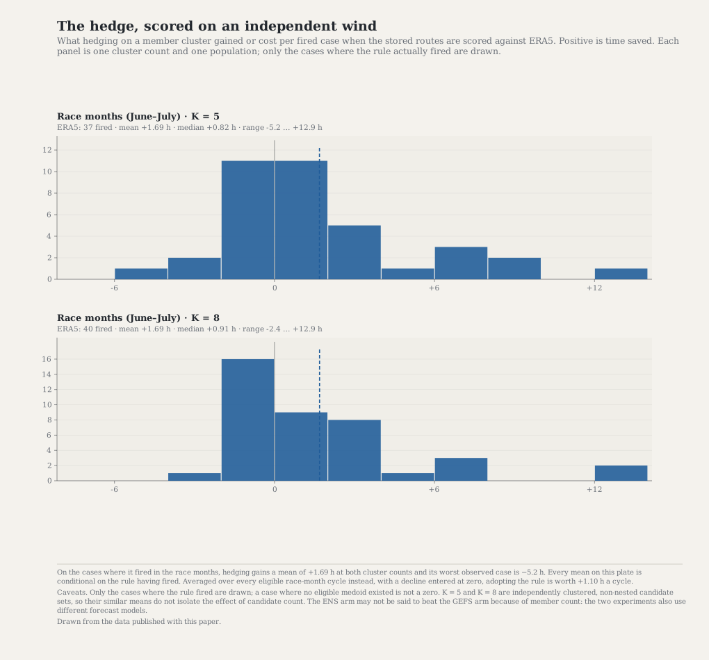
A navigator cannot choose only the cycles on which the rule works. The primary estimate therefore averages over every eligible cycle, with declines contributing zero. Within each cycle it averages the K = 5 and K = 8 records.
Table 14 — The hedge under ERA5, Transpac corpus. The primary interval uses a five-day block bootstrap. The other rows replace unscoreable firings with observed outcomes and are sensitivity scenarios, not mathematical bounds.
| Reading | Eligible cycles | Estimate | 95 % interval |
|---|---|---|---|
| Available-case policy estimate | 60 of 63 | +1.10 | [+0.41, +1.92] |
| Missing firings set to the worst observed outcome | 63 | +0.62 | [−0.07, +1.36] |
| Missing firings set to zero | 63 | +1.03 | [+0.39, +1.76] |
| Missing firings set to the best observed outcome | 63 | +2.06 | [+1.00, +3.35] |
The policy estimate is +1.10 h per eligible cycle [+0.41, +1.92]. At 8.9 kn, that is about 10 nm. Three cycles have no scoreable firing, and difficult weather may make both sailing and verification fail. Under the pessimistic observed-extreme scenario the estimate remains positive, but its interval includes zero. The scenarios cannot constrain an unobserved outcome outside the observed range.
7.2 What this means on the boat
The average gain is modest, but route geometry can separate early. A later recommendation may therefore point toward a route far from the boat's present line. This paper measures sustained geometric separation only through 150°W; it does not measure whether switching remains practical or cheap.
The rule also cannot choose a route absent from its stored candidates, and it cannot rescue a cycle in which the whole forecast distribution misses the relevant weather.
8. Pacific Cup 2026: one edition from start to finish
The archive-wide results combine thirteen editions. This section follows one edition instead: the 2026 Pacific Cup, with three starts and one July's weather. It is a worked example, not an independent test.
8.1 Three starts, three weather windows
For each gun, we route the canonical boat through that start's ERA5 weather and compare the hindsight optimum with the fleet-median line.
Table 15 — The three starts of the Pacific Cup 2026. Latitude is measured at 142°W. Positive offset means the hindsight optimum was north of the fleet median; positive replay time means the fleet-median line was slower. The ensemble columns describe the fifty member routes in the cycle preceding the gun.
| Start | Gun (UTC) | Boats | Optimum | Fleet median | Offset | Fleet IQR | Fleet replay gap | Members (mean ± sd) | Members min–max | Forecast lead |
|---|---|---|---|---|---|---|---|---|---|---|
| 1 | 2026-07-06T17:00Z | 9 | 28.89°N | 28.85°N | +2.8 nm | 2.08° | 8.0 h | 28.38 ± 0.64 | 27.11–29.66 | 17 h |
| 2 | 2026-07-07T18:00Z | 26 | 31.05°N | 28.82°N | +133.7 nm | 1.03° | 3.8 h | 28.20 ± 0.70 | 26.54–29.58 | 18 h |
| 3 | 2026-07-10T19:00Z | 13 | 28.81°N | 28.24°N | +33.9 nm | 0.44° | 5.4 h | 28.10 ± 2.82 | 23.52–35.31 | 19 h |
Figure 9 shows the three starts as sailed and the tracks of the seven qualifying division winners.
Scroll horizontally to inspect the chart labels.
Figure 9 — Pacific Cup 2026, the edition in one chart. The chart carries the three starts of one race: the orange lines are where the middle of each start’s fleet actually went, the blue lines are the hindsight optimum from that same gun, and the bracket on 142°W is the gap between them for the second start. Below, each dot is one scored division: the top row is how far north or south of its own rivals the winner sailed, the bottom row is how far it was from hindsight’s optimum, and the heavy mark is the mean of the seven. This edition illustrates measurements made across the larger archive; it is not an independent test. Across these seven qualifying divisions, the mean winner-versus-rivals latitude difference was +0.9 nm. Start 2’s hindsight optimum ran more than two degrees north of its fleet median, and every forecast member for that start lay south of the hindsight optimum.
Evidence and limits
- Start 2's optimum sat 134 nm north of the fleet median at 142°W; starts 1 and 3 sat 3 and 34 nm north.
- Across the seven scored divisions the winner sat +0.9 nm from its own rivals and -88.7 nm from the optimum.
- The High held station at 40.9°N 155.3°W with 1034.5 hPa at its centre through the decision band.
- The edition’s departure-day range was 21.2 h between its best and worst gun, against a thirteen-edition median of 29.2 h.
- Three starts, seven divisions and three forecast cycles: an illustration of measurements made elsewhere on thirteen editions, not an independent test of any of them.
- A corrected-time winner is selected on outcome, so its replayed geometry inherits whatever weather it found.
- The fleet median line is nobody's track, and it is shorter than any of them.
- The canonical boat is nobody's boat, and its elapsed times are not comparable with any published race result.
- The chart panel is Mercator, so the rhumb line is straight and a degree of latitude is sixty miles anywhere up the page; the scale bar names the latitude its miles are true at. Coastline: Natural Earth 1:10m, clipped to the corridor and committed with the rest of the data.
The second start supplies the useful case. Its hindsight optimum crossed 142°W at 31.05°N; the fleet median crossed at 28.82°N, 133.7 nm south. Before the gun, all fifty ensemble routes also remained south of the route later found in ERA5. A hedge among those candidates could not have selected the northern route.
That does not show that the fleet ignored a forecast. The archive does not record which products each navigator used or why each boat chose its line. It shows only that this forecast ensemble did not contain the later hindsight route.
8.2 What this edition can show
Across seven qualifying divisions, winners averaged +0.9 nm relative to their rivals' latitude and −88.7 nm from their starts' hindsight optima. Those values closely match the archive-wide results, but the same divisions are already part of that archive and do not provide an independent replication.
The edition is illustrative. Every solve uses the same hypothetical fifty-footer, not the boats that raced, and none of these comparisons identifies why a real boat won.
9. Discussion
9.1 The largest variation is assigned before the start
The results describe different quantities and cannot be added. The clearest ordering is still useful. For the same boat within one edition, the best-to-worst start-day range is 29.2 h [18.5, 47.7]. That is a range, not the effect of assigning a particular date, but it shows the scale of weather differences across a staggered schedule.
Route value depends on the comparator. Replaying each division winner against its actual rivals gives +0.02 h [−1.12, +1.16]. A speed-matched composite against hindsight is also unresolved. The whole-fleet composite gives +5.00 h, but its start-level interval crosses zero while its edition-resampled interval barely clears it. That comparison mixes boat speeds, uses a line nobody sailed, and carries resampling error of the same order as its estimate.
Winners did record shorter tracks, averaging 12.0 nm less [1.5, 22.6] over the ground. The association may reflect efficient steering, better positioning in the weather, or both; it does not establish the cause. Certificate scatter and the ensemble hedge belong to still different comparisons. Sister ships differ by 1.60 % in the ORC archive, while the forecast policy gains +1.10 h per eligible cycle [+0.41, +1.92]. Common units make their scale visible, not interchangeable.
9.2 A climatology cannot locate one week
The fixed-boat archive detects no July trend in elapsed time, distance or route latitude over the satellite era. The fitted elapsed-time change is +10.1 h [−9, +29]. This does not show that the Pacific climate has not changed; it says that this navigational integral has no detected trend in the declared archive.
Departure date varies much more. Optimal elapsed time differs by 26.4 h on average between departures five days apart and by 45.0 h across 6–16 July. Pressure does not repair the scale mismatch: its out-of-sample position error is 117.6 nm, against 77.3 nm for latitude. Pressure describes where a route went, but it did not make a better almanac.
9.3 Fleets adjust between years, not detectably between starts
Fleet latitude and hindsight latitude move together across editions. On Transpac their correlations range from +0.673 to +0.945. Within editions, after matching each start to its speed band, no corresponding start-to-start relationship is detected. Fleets respond to the character of a year; the archive does not show that divisions starting a few days apart follow the optimum's short-term movement.
Winners occupy no detectable special lane and are not detectably closer to hindsight than their rivals. The fleet as a whole nevertheless sails roughly 60–90 nm south of the flat-water hindsight optimum. That should not be called navigational error. Hindsight knows the weather that followed, while crews choose under forecast uncertainty and with physics the model omits.
9.4 Certificate variation is large enough to measure
Matched sister ships differ by 1.60 % [1.50, 1.69] in GPH, while one boat's de-trended year-to-year movement is 0.29 % [0.285, 0.300]. The first includes real differences in sails, propeller, keel, loading and declared configuration; it is not certificate error or evidence of gaming. Winners also sit near the middle of their observed rating bands. These results measure rating variation, not the effect of changing a boat's certificate or rating system.
9.5 What this requires from a routing tool
A useful routing interface should show candidate route families and their downside before the weather is known. It may show where candidates stop reconverging within the assessed scan, but it must not call that point irreversible: this study stops at 150°W and does not measure switching cost. Because winners did not occupy a special strategic lane but often recorded shorter tracks, the tool should also help a crew hold, monitor and reassess a chosen route rather than present one optimum with unsupported precision.
9.6 Relation to prior work
Minimum-time routing follows the isochrone tradition of James (1957) and later implementations (Walther et al., 2016). Ensemble routing with explicit risk predates this study (Philpott & Mason, 2001; Tagliaferri et al., 2014), as do multi-year rerouting experiments (Dupuy et al., 2023) and comparisons between sailed tracks and computed optima (Forsberg et al., 2024; Goto et al., 2024). Teeters and Honey (2025) provide the closest operational precedent by routing representative fleets through forecast and historical weather for race-specific ratings. This paper applies those established ideas to a fixed-boat climate archive, tracked Hawaii fleets, and independent verification of an ensemble selection policy.
9.7 Limits of the evidence
- The quantities cannot be pooled. Start-day ranges, route differences, forecast-cycle means, division margins and certificate spreads use different populations and counterfactuals.
- Hindsight is not operational. It knows the verifying weather, so a fleet-to-hindsight difference is not recoverable time available to a navigator.
- Replayed hours carry resampling error. Latitude and over-ground distance come directly from geometry; elapsed-time comparisons add verification replay and meridian-grid discretization.
- Forecast results have missing outcomes and retrospective choices. Observed-extreme fills are sensitivity scenarios, not bounds, and the policy settings were selected on the available archive.
- Route separation is bounded by the scan. It is sustained only through 150°W and does not measure switching cost, regret or irreversibility.
- The route model omits important physics. Flat-water polars omit waves and squalls, and most solves omit current. Their directional biases have not been established.
- The fleet, winner, start and certificate analyses are observational. No boat was assigned a route, start or certificate, so associations must not be read as effects.
10. Conclusion
A Hawaii race presents one physical trade: the shortest route runs toward the light air around the North Pacific High, while more wind usually costs more distance. The measurements in this paper describe parts of that trade. They do not add to one formula for winning.
No route-climate trend is detected at the scale of this archive. The fitted satellite-era change in optimal elapsed time is +10.1 h [−9, +29]. Weather within one July is much larger: departures five days apart differ by 26.4 h on average for the same boat and solver. Climatology is background; the start week's forecast still determines the problem.
Winners do not occupy a detectable special lane. Replaying each winner against its own rivals gives +0.02 h [−1.12, +1.16]. Winners nevertheless record tracks averaging 12.0 nm shorter [1.5, 22.6]. That association does not establish whether sailing less distance caused the result or followed from better positioning in the weather.
The ensemble hedge gains +1.10 h per eligible cycle [+0.41, +1.92], about 10 nm at 8.9 kn. Missing outcomes make the pessimistic sensitivity interval include zero. Candidate routes may remain separated through 150°W, but this paper does not measure a point of no return.
Matched sister ships differ by 1.60 % in the ORC archive and race-relevant designs by 1.83 %, roughly four hours on the reference passage. Those differences include real configuration variation and are not rating error. The practical sequence is simpler: understand the usual route, solve the actual start and forecast, inspect the forecast distribution, keep the sailed path short when the weather permits, and know the boat and certificate. Each step addresses a measurable quantity; none alone explains why a boat won.
11. References
Carver, R. W., & Merose, A. (2023). ARCO-ERA5: an analysis-ready cloud-optimized reanalysis dataset. 22nd Conference on Artificial Intelligence for Environmental Science, Denver, CO, American Meteorological Society, 4A.1. https://ams.confex.com/ams/103ANNUAL/meetingapp.cgi/Paper/415842
Chassignet, E. P., Hurlburt, H. E., Smedstad, O. M., Halliwell, G. R., Hogan, P. J., Wallcraft, A. J., Baraille, R., & Bleck, R. (2007). The HYCOM (HYbrid Coordinate Ocean Model) data assimilative system. Journal of Marine Systems, 65(1–4), 60–83. https://doi.org/10.1016/j.jmarsys.2005.09.016
Dupuy, M., Letournel, L., Paakkari, V., Rongère, F., Sarsila, S., & Vuillermoz, L. (2023). Weather routing benefit for different wind propulsion systems. Journal of Sailing Technology, 8(1), 200–217. https://doi.org/10.5957/jst/2023.8.11.200
Forsberg, B., Pashami, S., Corona, E., Pezzoli, F., Sütfeld, L. R., & Marimon Giovannetti, L. (2024). A data-driven race strategy tool for Olympic sailing competitions. Journal of Sailing Technology, 9(1), 78–93. https://doi.org/10.5957/jst/2024.9.1.78
Goto, Y., Weimerskirch, H., Fukaya, K., Yoda, K., Naruoka, M., & Sato, K. (2024). Albatrosses employ orientation and routing strategies similar to yacht racers. Proceedings of the National Academy of Sciences, 121(23), e2312851121. https://doi.org/10.1073/pnas.2312851121
Hagiwara, H., & Spaans, J. A. (1987). Practical weather routing of sail-assisted motor vessels. Journal of Navigation, 40(1), 96–119. https://doi.org/10.1017/S0373463300000333
Hersbach, H., Bell, B., Berrisford, P., Hirahara, S., Horányi, A., Muñoz-Sabater, J., Nicolas, J., Peubey, C., Radu, R., Schepers, D., Simmons, A., Soci, C., et al. (2020). The ERA5 global reanalysis. Quarterly Journal of the Royal Meteorological Society, 146(730), 1999–2049. https://doi.org/10.1002/qj.3803
Honey, S. (n.d.-a). Stan Honey's weather advice. Pacific Cup Yacht Club knowledge base. https://pacificcup.org/kb/stan-honeys-weather-advice
James, R. W. (1957). Application of wave forecasts to marine navigation. U.S. Navy Hydrographic Office, Washington, DC, 92 pp. (Reprinted 1959 and 1975 by the U.S. Naval Oceanographic Office.) Defense Technical Information Center accession AD0158747. https://trid.trb.org/view/388400
Leutbecher, M., & Palmer, T. N. (2008). Ensemble forecasting. Journal of Computational Physics, 227(7), 3515–3539. https://doi.org/10.1016/j.jcp.2007.02.014
Molteni, F., Buizza, R., Palmer, T. N., & Petroliagis, T. (1996). The ECMWF ensemble prediction system: methodology and validation. Quarterly Journal of the Royal Meteorological Society, 122(529), 73–119. https://doi.org/10.1002/qj.49712252905
Offshore Racing Congress (2026). ORC VPP Documentation 2026. Offshore Racing Congress. https://orc.org/uploads/files/Rules-Regulations/2026/ORC-VPP-Documentation-2026.pdf
Philpott, A., & Mason, A. (2001). Optimising yacht routes under uncertainty. 15th Chesapeake Sailing Yacht Symposium, Annapolis, MD, SNAME, paper D011S001R009. https://doi.org/10.5957/CSYS-2001-009
Rockafellar, R. T., & Uryasev, S. (2000). Optimization of conditional value-at-risk. The Journal of Risk, 2(3), 21–41. https://doi.org/10.21314/JOR.2000.038
Taburet, G., Sanchez-Roman, A., Ballarotta, M., Pujol, M.-I., Legeais, J.-F., Fournier, F., Faugere, Y., & Dibarboure, G. (2019). DUACS DT2018: 25 years of reprocessed sea level altimetry products. Ocean Science, 15(5), 1207–1224. https://doi.org/10.5194/os-15-1207-2019
Tagliaferri, F., Philpott, A. B., Viola, I. M., & Flay, R. G. J. (2014). On risk attitude and optimal yacht racing tactics. Ocean Engineering, 90, 149–154. https://doi.org/10.1016/j.oceaneng.2014.07.020
Teeters, J., & Honey, S. (2025). Weather based scoring of sailboat races. Journal of Sailing Technology, 10(1), 314–328. https://doi.org/10.5957/jst/2025.10.1.314
Walther, L., Rizvanolli, A., Wendebourg, M., & Jahn, C. (2016). Modeling and optimization algorithms in ship weather routing. International Journal of e-Navigation and Maritime Economy, 4, 31–45. https://doi.org/10.1016/j.enavi.2016.06.004
Attributions
ERA5 (ARCO-ERA5, Copernicus Climate Change Service). Licensed CC-BY-4.0. Required statement: "Contains modified Copernicus Climate Change Service information 2026. Neither the European Commission nor ECMWF is responsible for any use that may be made of the Copernicus information or data it contains."
ECMWF open data (ENS and HRES). Licensed CC BY 4.0 subject to the ECMWF Terms of Use, which require the statement that "this document/data/output/Results is/are based on data and products of the European Centre for Medium-Range Weather Forecasts (ECMWF)".
Yellowbrick race-tracker archive. Public race coverage of eight Transpac editions (2011–2025) and five Pacific Cup editions (2016–2026).
HYCOM (HYCOM Consortium; Naval Research Laboratory and partners). Global ocean analysis, hindcast and operational output. Every field used here was subset, resampled and integrated by this work's own tooling and is therefore modified.
Transpacific Yacht Club race programmes. The club's own official programmes, 1936–2025. They remain the club's copyright; the paper quotes only short passages with the edition and page they came from.
ORC certificates. The public archive of Offshore Racing Congress certificates for 2019–2025. Certificates are the certifying authority's published measurements; nothing here is issued, endorsed or checked by them.
Competing interests
WX Navigator is a commercial weather-routing product built by the author. Section 7 evaluates the ensemble-hedging rule implemented by that product.